728x90
반응형
심층신경망_분류데이터사용
- 입력계층의 출력크기 64
- 은닉계층의 출력크기 32
- 나머지는 ?
- 콜백함수 모두 적용
- 옵티마이저 모두 적용해보기
- 정밀도, 재현율, f1-score, confusion_matrix출력
작성한 코드
- 라이브러리 정의
-
import pandas as pd from sklearn.preprocessing import StandardScaler from sklearn.model_selection import train_test_split import tensorflow as tf from tensorflow import keras from sklearn.metrics import precision_score, recall_score, f1_score, confusion_matrix from sklearn.metrics import ConfusionMatrixDisplay - 데이터 가져오기
- 데이터프레임 변수 : data
- 데이터 읽어들이기
- 종속변수 : 주택가격
- 주택가격이 연속형 데이터이므로 회귀데이터
data = pd.read_csv("./data/08_wine.csv") data.head(1) - 독립변수(X)와 종속변수(y)로 분리하기
X = data.iloc[:,:-1] y = data["class"] X.shape, y.shape - 데이터 정규화
- X_scaled 변수명 사용
ss = StandardScaler() ss.fit(X) X_scaled = ss.transform(X) X_scaled.shape - 훈련 : 테스트 데이터로 분류하기 (8 : 2)
- 사용 변수 : X_train, X_test, y_train, y_test
X_train, X_test, y_train, y_test = train_test_split(X_scaled, y, test_size=0.2, random_state=42) print(f"{X_train.shape} : {y_train.shape}") print(f"{X_test.shape} : {y_test.shape}") - 함수 생성
def model_d(): model = keras.models.Sequential() model.add(keras.layers.Dense(64,input_shape=(3,),activation='sigmoid')) model.add(keras.layers.Dense(32,activation='sigmoid')) model.add(keras.layers.Dense(1,activation='sigmoid')) return model def model_f(model, opt, epoch) : model.compile(optimizer = opt, loss="binary_crossentropy", metrics="accuracy") checkpoint_cb = keras.callbacks.ModelCheckpoint( "./model/best_model.h5", save_best_only = True) early_stopping_cb = keras.callbacks.EarlyStopping( patience=2, restore_best_weights=True) history = model.fit( X_train, y_train, epochs=epoch, verbose=1, validation_data=(X_test, y_test), callbacks=[checkpoint_cb, early_stopping_cb]) return history - 함수 호출
''' 함수 호출하기 ''' ''' 옵티마이저를 리스트로 정의하기 ''' optimizers = ["sgd", "adagrad", "rmsprop", "adam"] history_loss = {} history_acc = {} ''' 옵티마이저의 학습방법을 반복하여 성능 확인하기 ''' for opt in optimizers : print(f"--------------------------{opt}--------------------------") model = model_d() history = model_f(model, opt, 100) history_loss[min(history.history['val_loss'])] = opt history_acc[min(history.history['val_accuracy'])]= opt print(f"최적의 학습기법 : {history_loss[min(history_loss.keys())]} / 손실율 : {min(history_loss.keys())} ") print(f"최적의 학습기법 : {history_acc[max(history_acc.keys())]} / 정확도 : {max(history_acc.keys())}")
- 모델 생성
model = model_d() model_f(model, "adam", 100) - 예측하기
y_pred = model.predict(X_test) for i in range(len(y_pred)): if y_pred[i] > 0.5: y_pred[i] = 1 else: y_pred[i] = 0 y_pred
- 정밀도, 재현율, f1-score, confusion_matrix 출력
precision = precision_score(y_test,y_pred)
recall = recall_score(y_test,y_pred)
f1 = f1_score(y_test,y_pred)
cm = confusion_matrix(y_test,y_pred)
print("Precision:", precision)
print("Recall:", recall)
print("F1 Score:", f1)
print("Confusion Matrix:", cm)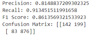
- 오차행렬도 그리기
disp = ConfusionMatrixDisplay(confusion_matrix =cm)
disp.plot()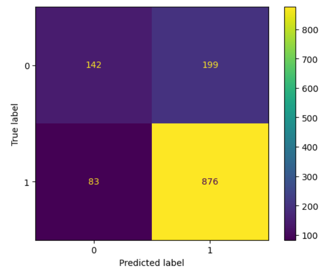
강사님 코드
- 라이브러리 정의
import pandas as pd from sklearn.preprocessing import StandardScaler from sklearn.model_selection import train_test_split import tensorflow as tf from tensorflow.keras.models import Sequential from tensorflow.keras.layers import Dense from sklearn.metrics import accuracy_score, precision_score, recall_score, f1_score, confusion_matrix - 데이터 불러들이기
data = pd.read_csv("./data/08_wine.csv") data.head(1) - 데이터 정규화
ss = StandardScaler() ss.fit(X) X_scaled = ss.transform(X) X_scaled.shape - 훈련 : 검증 : 테스트 데이터로 분류하기 (6 : 2 : 2)
X_train, X_temp, y_train, y_temp = train_test_split(X_scaled, y,
                                                   test_size=0.4,
                                                   random_state=42)

X_val, X_test, y_val, y_test = train_test_split(X_temp, y_temp,
                                                   test_size=0.5,
                                                   random_state=42)

print(f"훈련 데이터 {X_train.shape} : {y_train.shape}")
print(f"검증 데이터 {X_val.shape} : {y_val.shape}")
print(f"테스트 데이터 {X_test.shape} : {y_test.shape}")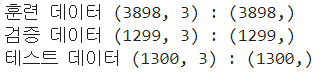
- 모델 생성
model = Sequential() model - 계층 생성
'''
입력 은닉 계층에는 softmax빼고 다른 함수 다 들어갈 수 있다.
softmax는 출력 계층에만 들어간다
'''

'''
<입력계층>
 - 64 : 출력크기
 - activation=relu0 : 활성화 함수. relu는 0보다 크면 1, 0보다 작으면 0
 - input_dim=3 : 입력 특성의 갯수 (input_shape 대신에 사용가능)
'''
model.add(Dense(64, activation="relu", input_dim=3))

'''
Dropout은 과대적합 나올때 은닉계층 전에 사용하여 모델을 덜 똑똑하게 만들어버린다.
은닉계층이 두개라면 은닉계층 전에 사용할 수 있기 때문에 dropout또한 2개 사용 가능하다.
'''

'''
<은닉 계층>
'''
model.add(Dense(32, activation="relu"))

'''
<출력 계층>
 - sigmoid : 이진분류이기 때문에 0.5를 기준으로 0 또는 1로 나뉘는 sigmoid 사용
'''
model.add(Dense(1, activation="sigmoid"))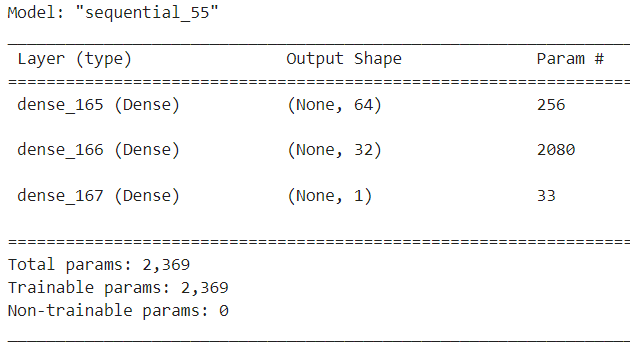
- 모델 설정하기
''' - 이진분류 이므로 binary_crossentropy 사용 - 다중분류 : sparse ''' model.compile(loss="binary_crossentropy", optimizer="adam", metrics=["accuracy"]) - 모델 훈련시키기
model.fit(X_train, y_train, epochs=100,
         validation_data=(X_val, y_val))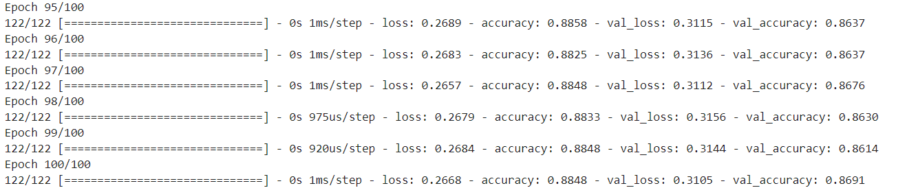
- 성능검증
loss, acc = model.evaluate(X_test, y_test)
loss, acc
- 예측하기
y_pred = model.predict(X_test)
y_pred
이 값을 종속변수와 비교하기 위해 1 또는 0으로 바꿔야 함
 - 평가를 위해서 예측값을 종속변수의 범주 형태(0 or 1)로 변환하기
''' True = 1, False = 0 '''
base = 0.5
binary_pred = (y_pred > base).astype(int)
binary_pred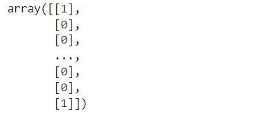
- 성능 평가
precision = precision_score(y_test, binary_pred)
recall = recall_score(y_test, binary_pred)
f1 = f1_score(y_test, binary_pred)
precision, recall, f1
- 매트릭스 확인
conf_matrix = confusion_matrix(y_test, binary_pred)
conf_matrix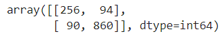
728x90
반응형
'Digital Boot > 인공지능' 카테고리의 다른 글
| [인공지능][DL] Deep Learning - 심플 순환신경망(Simple RNN) (1) | 2024.01.05 |
|---|---|
| [인공지능][DL] Deep Learning - 퍼셉트론(Perceptron) 모델 (0) | 2024.01.05 |
| [인공지능][DL] Deep Learning - 심층신경망 훈련 및 성능향상 (2) (2) | 2024.01.04 |
| [인공지능][DL] Deep Learning - 심층신경망 훈련 및 성능향상 (1) | 2024.01.03 |
| [인공지능][DL] Deep Learning 실습 - 신경망계층 추가방법 및 성능향상방법 (1) | 2024.01.03 |